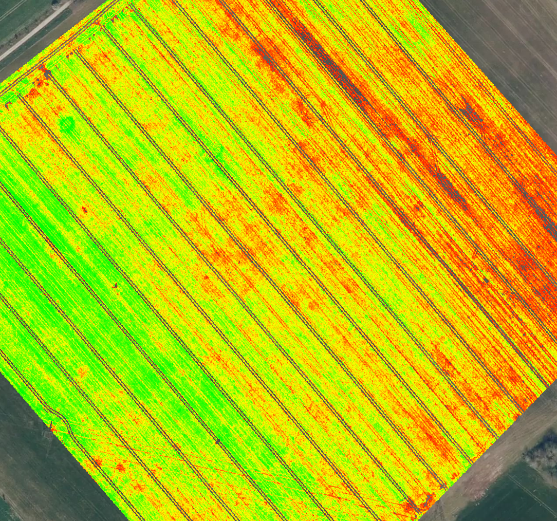
The goal of this project is to obtain a Normalized Difference Vegetation Index (NDVI) index map of a Winter Wheat field using the DJI Phantom 4 multispectral camera that captures Green, Red, Blue, Red edge, and NIR wavelengths. The same workflow is explained in our PIX4Dfields tutorial videos. 📺🌱
IN THIS ARTICLE
Download example images
Create a project and import images
Process and trim
Generating an index
Understanding the NDVI
Creating a zonation for variable rate application
Download example images
|
Dataset size
|
5 GB |
| Average Ground Sampling Distance (GSD) | 6.2 cm / 2.44 in. |
| Area covered | 46.5 ha / 114 acres. |
| Image acquisition plan | 1 flight, grid flight plan. |
| Drone and camera | DJI Phantom 4 Multispectral, Multispectral camera |
| Reflectance panel/target | Micasense |
| Download example images | |
Download example imagery and unzip the folder:
- Right-click on the "01_Images.7z" file.
- Click Extract all

- Click Extract.
Create a project and import images
To create a new project:
- On the dashboard, click + New Project or the “plus” symbol at the bottom right corner of the window.

- A new window with a background satellite image appears, displaying either the default location or where the last project was processed.
- Click the pen symbol beside the default name of the project to rename the project.
To import images captured by drone:
- Images option allows you to select several images, Folder allows you to import a complete folder simultaneously.
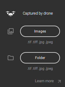
- Click Folder, select the unzipped folder "01_Images", and click Open.
- When processing a camera that captures RGB and Multispectral (i.e Parrot Sequoia, Mavic 3 Multispectral, Phantom 4 Multispectral), the Image type selection menu will appear:

- Choose .tiff to process the Multispectral images, or choose .jpg to process RGB images.
- In this case, please choose .tiff.
Recommended tutorial video 📺:
Process and trim
After importing the first images, the Processing options menu appears. For more information: Processing options.
Fast Processing is the default processing option as it gives rapid results with minimal compromise in the accuracy of outputs. Fast processing still offers the best option for generating an orthomosaic, index maps, and DSM with sufficient resolution for most farming applications.
Accurate processing generates a highly detailed height model and a more accurate orthomosaic (better geolocation of pixels, i.e., less potential for distortions, especially around sudden elevation changes). However, the more complex processing algorithm will increase processing times. This is ideal for trial plots, spot applications, and terrain analysis.
- Choose Fast processing.
- Click Apply.
- If more images need to be added, click Import images or Import folder again.
- If the Processing settings need to be changed, click the Settings icon beside the Start processing button.
- To begin the process, click Start processing.
Once processing is completed, click on the Orthomosaic and the Surface Model to display them on the interface.
The Orthomosaic contains the available bands. In this case, it contains the Red, Blue, Green, NIR, and RedEdge bands.
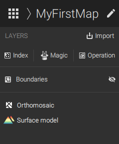
Before generating an index, it is recommended to trim the layer.
Click the Boundaries layer on the left board above the layer list to enter the boundaries mode.
- To draw a field boundary, click the Draw boundary icon in the left corner of the map.
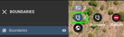
- Select Boundary. Note that obstacles can be created as well.
- Left-click to start drawing.
- For more information: Field boundaries and obstacles - PIX4Dfields.
 import after finishing the first processing.
Generating an index
To generate a vegetation index:
- Click Index above the Layers Menu.

- The INDEX GENERATOR tool opens
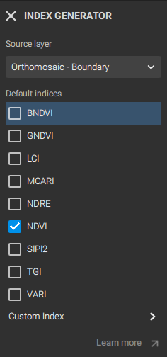
- Select the Orthomosaic as the Source layer.
- Select the Vegetation Index you want to generate by checking the corresponding boxes.
- Click Generate.
Congratulations on your first Vegetation Index map 🚀🌱!
For more information: How to generate a vegetation index - PIX4Dfields.
Recommended tutorial video 📺:
Understanding the NDVI
The NDVI (Normalized Difference Vegetation Index) is sensitive to chlorophyll content.
Healthy vegetation absorbs most of the visible light that hits it and reflects a large portion of the near-infrared light. As a result, healthy vegetation will have a high NDVI value.
The NDVI scale ranges from -1 to +1. This scale is designed to represent different types of land cover and vegetation health or density. Here's a brief overview of what values within this range typically indicate:
- Values close to +1: High NDVI values (close to +1) indicate dense green leaves and are typically associated with healthy, vigorous vegetation. This is because healthy vegetation reflects more near-infrared (NIR) light and absorbs more visible light.
- Values close to 0: NDVI values around 0 indicate barren areas of rock, sand, or snow, where there is little difference in the reflectance between the red and NIR wavelengths, suggesting minimal vegetation.
- Values close to -1: Negative NDVI values (close to -1) are possible but less common and can occur when the reflectance in the red wavelength is greater than the reflectance in the NIR wavelength. This situation might be observed in water bodies, where the absorption of NIR is higher than the absorption of visible light, resulting in negative NDVI values.
It's important to note that NDVI values are influenced by the specific characteristics of the area being observed, including the type of vegetation, the stage of growth, and the presence of any stress factors (like water availability or diseases). Here's a more detailed breakdown of the NDVI value obtained in the previously provided data:

- -1.0 to 0.0: There are no pixels with these values, as it's mainly related to non-vegetated surfaces, (water, snow, clouds, etc.)
- 0.0 to 0.5: Bare soil, as evident from the machine tire marks.

- 0.5 to 0.7: Non-healthy vegetation, low plant density.
- 0.5 to 0.7: Healthier vegetation.
- 0.9 to 0.973: Dense vegetation, healthy crops at peak vitality.
Creating a zonation for variable rate application
The next step involves utilizing the Targeted Operation feature to transform the Vegetation Index into a machine-readable format.
The final map is used for agricultural operations on the field and read by a tractor terminal or a spraying drone. It combines geographic locations with rate values, instructing the machine on where to apply what amount of product.
For further details: How to create zonations for targeted spraying - PIX4Dfields